Value Function Approximation

Algorithm Characteristics

• Model-Free
• Value-Based
• Incremental
• Function Representation

 

 

 

1. State Value Estimation

就是在做 Policy Evaluation，但是没法 search for optimal policy

 

 

1.1 Problem Formulation

Given

• $v_\pi(s) \longrightarrow$ Ground Truth State Value
• $\hat{v}(s, w) \longrightarrow$ Function to approximate State Value, where $w$ is its weight

Goal

• Find an optimal weight $w$ such that $\hat{v}(s, w)$ can best approximate $v_\pi(s)$ for every $s$

 

 

1.2 Objective Function

一共有三种 Objective Function，不过我们之后暂且先在 True Value Error 的基础上探讨

 

1.2.1 True Value Error

Value Function Approximation 这种方法所用的目标函数如下

关于 notation：$\lVert x \rVert_D^2 = x^TDx$

where state random variable $S \in \mathcal{S}$

求 Expectation 本质上是求关于该 random variable 的 average，因此需要选定 $S$ 的 probability distribution

• Uniform Distribution

  即简单粗暴地认定 all the states are equally important，设每个 state 的概率均为 $\frac{1}{\abs{S}}$，此时

  这种做法显然完全不尊重 Markov Process 的 dynamics

• Stationary Distribution

  也叫 Steady-State Distribution，描述的是一个 Markov Process 的 long-run behavior，设置每个 state 的概率为 $\{d_\pi(s)\}_{s\in\mathcal{S}}$

  where $\{d_\pi(s)\}_{s\in\mathcal{S}}$ denotes the stationary distribution of the Markov Process under policy $\pi$

  此时

  其实就是拿一个 Policy $\pi$ 去疯狂 rollout，理论上次数够多，那么每个 state 被访问到的概率就会慢慢收敛到固定值上，被访问次数更多的 state 在 objective function 中就能获得更高的权重

  

  上图中，左图为一个 4 个 states 的 grid world 和 $\epsilon$-greedy policy ($\epsilon = 0.5$) ，右图的曲线表示随 step 变化 4 个 states 被访问到的概率，图中最右侧不同颜色的 $\ast$ 代表着 4 个 states 被访问到的 probability 的理论值

  这个理论值也是可以计算的，recall the matrix-vector form of Bellman Expectation Equation and State-Transition Matrix

  where $n$ is the number of states，上图中右图每 step 一次就会更新一次 $d_\pi = [d_\pi(s_1), d_\pi(s_2), \cdots, d_\pi(s_n)]^T \in \R^n$

  直到 step 够久了，$d_\pi$ 就会变成一个 fixed point（或者说 converge to fixed value）

  例子中的 state transition matrix 是

  计算出的 $d_\pi$ 理论值为

 

1.2.2 Bellman Error

如果 $\hat{v} \to v_\pi$，且 $v_{\pi} = r_{\pi} + \gamma P_{\pi}v_{\pi}$ 那么

where

 

1.2.3 Projected Bellman Error

有时候由于所选择的 $\hat{v}$ 的结构上的因素，可能永远都会是 $\hat{v}(w) \not= T_\pi(\hat{v}(w)$；此时如果只用 Bellman Error，那么 $J(w)$ 永远无法逼近 0

where $M \in \R^{n\times n}$ is the orthogonal projection matrix that geometrically projects any vector onto the space of all approximations

 

 

1.3 Optimization Algorithm

We can use Gradient Descent to minimize the Objective Function

where

可以用 stochastic gradient 替代计算 expectation 的步骤

由于需要 True State Value $v_\pi(S)$，所以这个算法实际上是不可行的，但是还有其它方案

• Monte Carlo

  Use $v_\pi(s_t) \approx g_t$，where $g_t$ is the discounted return starting from state $s_t$ in the episode

• Temporal Difference

  Use $v_\pi(s_t) \approx r_{t+1} + \gamma\hat{v}(s_{t+1}, w_t)$ by the spirit of TD method

  需要注意的是，这个公式 minimize 的 objective function 本质上并不是 1.2.1 True Error，而是 1.2.3 Projected Bellman Error

 

 

1.4 Function Approximator

如何选择 $\hat{v}(s, w)$ ？

• Neural Network

  如今被广泛使用的选择，用 NN 的 nonlinearity 把它当成一个万能的 function approximator，这在 3.2 Deep Q-Learning (DQN) 里会详细聊

• Linear Function

  这个算是前朝遗物，但是能帮助理解

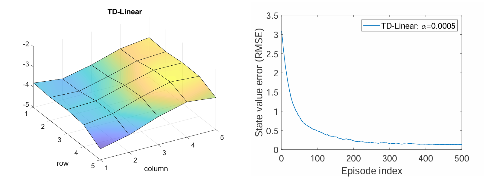
  where $\phi(s)$ is the feature vector，它可以是 polynomial basis，可以是 Fourier basis ... 总之可选项很多。此时

  代入前面提到的 TD 版的 Gradient Descent 后，就能得到所谓的 TD-Linear 算法

  而 feature vector $\phi(s)$ 的选择会在很大程度上影响 TD-Linear 的效果

  不如说 function approximator 的结构 会对最终近似的效果产生影响

  就像 Linear Function 的结构决定了它的近似上限永远不会比 Neural Network 高

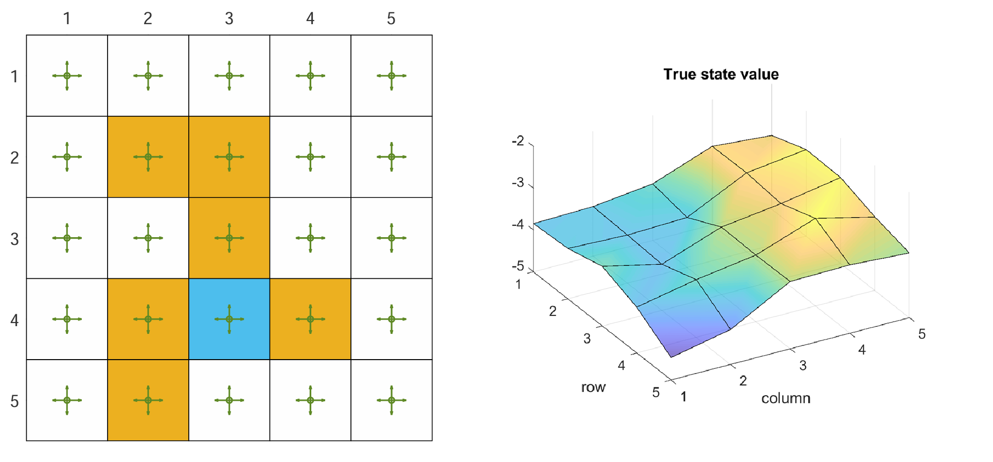
  假设要 evaluate 如下的 Policy：25 个 state，5 个 action，每个 action 的概率都是0.2

  

  • Feature Vector Selection [1]:

    the approximated state Value is

    效果为

    

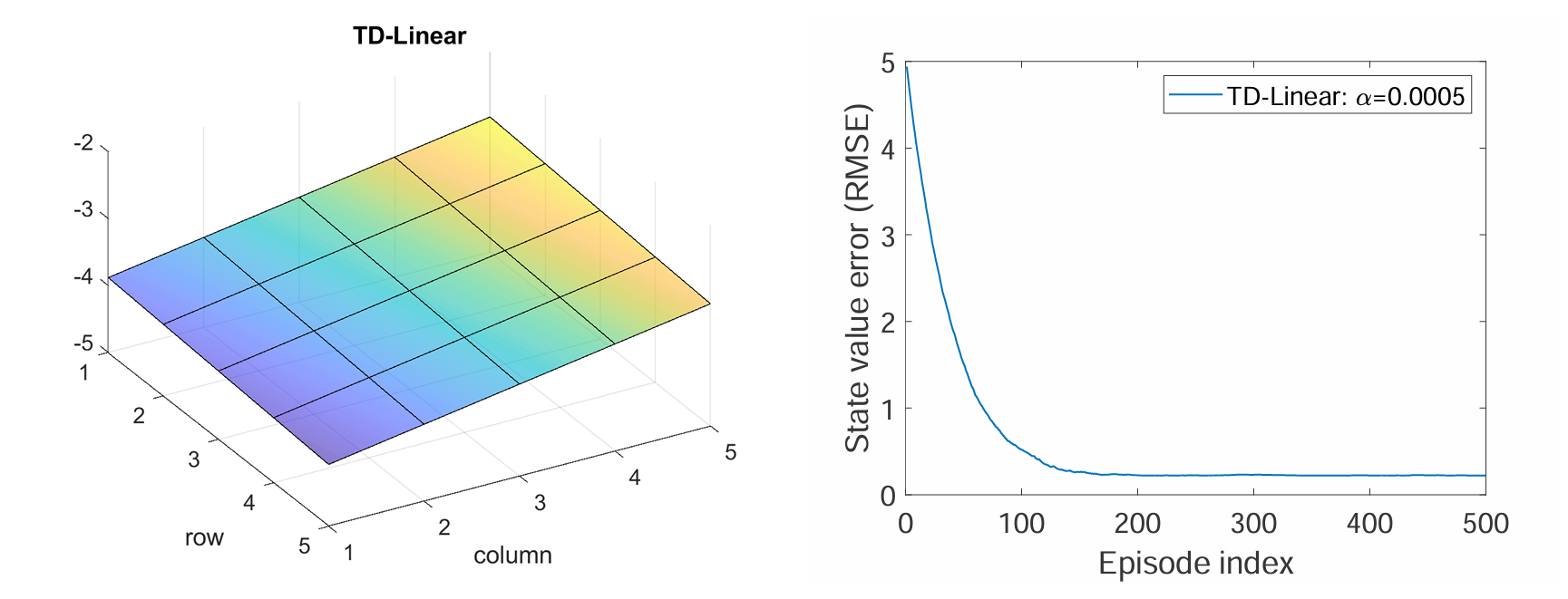
  • Feature Vector Selection [2]:

    the approximated state Value is

    效果为

    

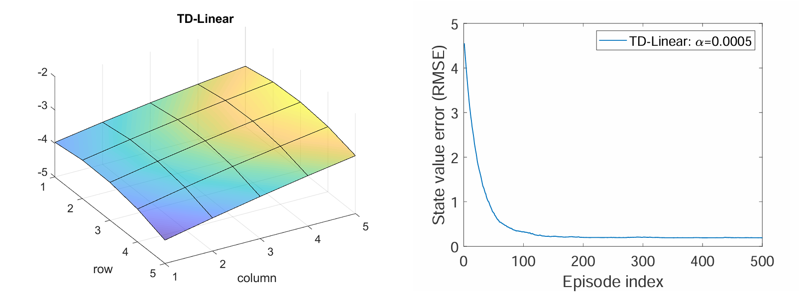
  • Feature Vector Selection [3]:

    the approximated state Value is

    效果为

    

 

 

 

2. Action Value Estimation

• 一般意义上的 Function Approximation for Action Value Estimation
• 以 Temporal Difference 的两个对应算法为基础
• 可以 search for optimal policy

 

 

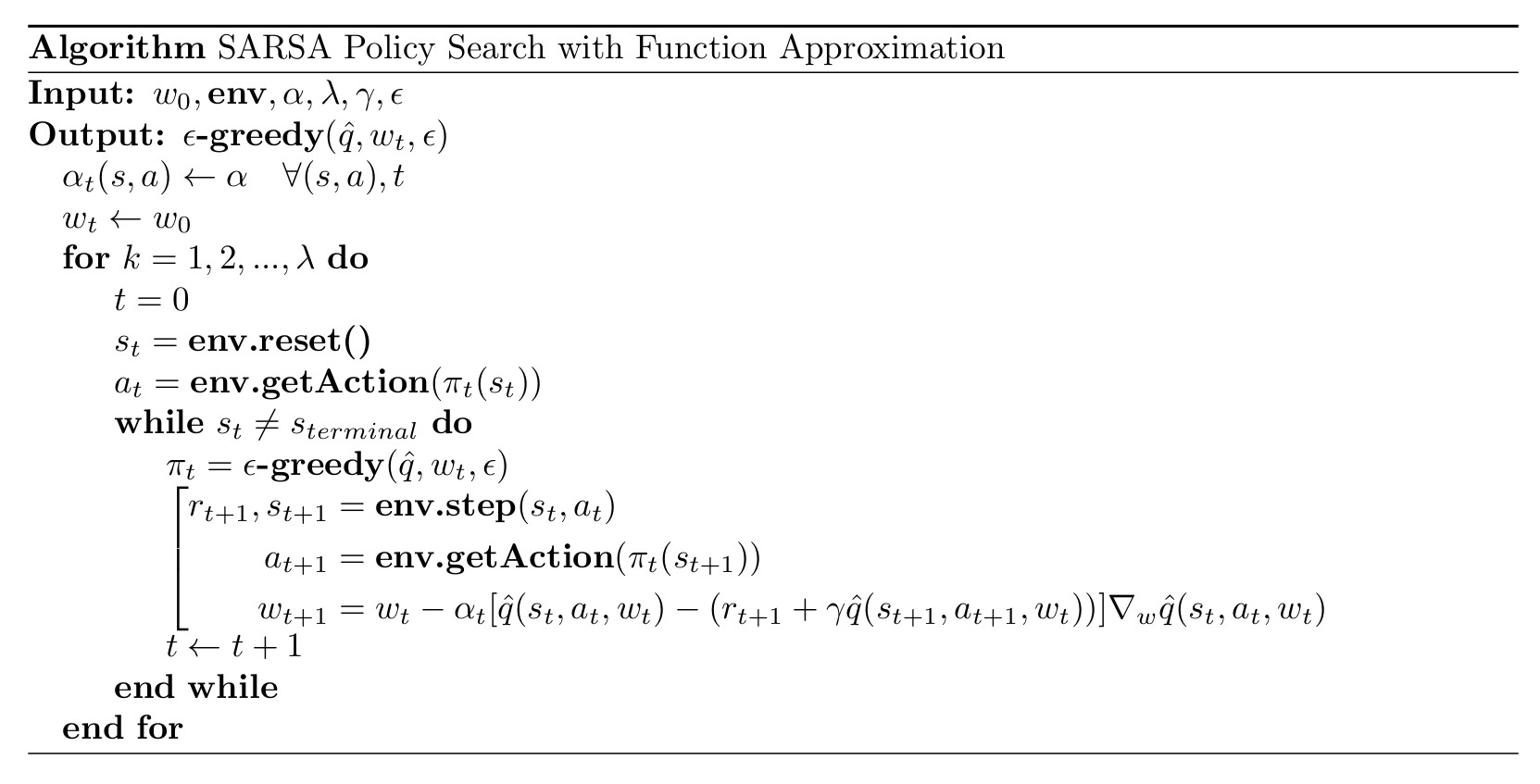
2.1 Sarsa

Sarsa with value function approximation，estimate action value

原理和前文 TD 版的 state value estimation 是差不多的，无非就是把 state value $v$ 替换成 action value $q$

以下是 pseudo code

 

 

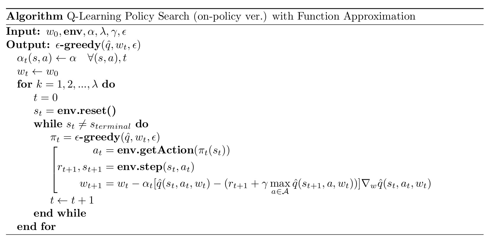
2.2 Q-Learning

Q-Learning with value function approximation，estimate optimal action value

和 Sarsa 版的区别是 TD Target 的 $\hat{q}$ 被替换成了 $\max_{a\in\mathcal{A}}\hat{q}$

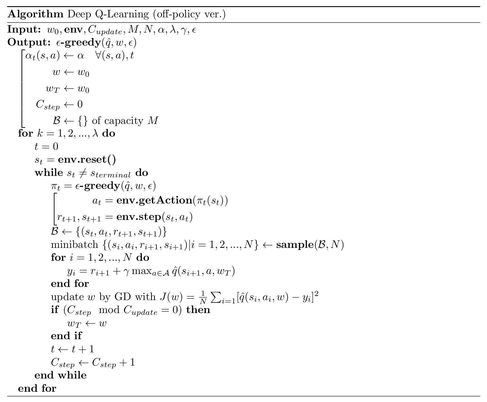
以下是 pseudo code

 

 

3. Deep Q-Network (DQN)

Deep Q-Learning / Deep Q-Network 是最早最成功地把 Deep Neural Network 引入 RL 的方法

 

3.1 Objective Function

Recall that Q-Learning aims to solve the Bellman Optimality Equation

但这个 objective function 是不能直接拿来用的，因为如果此时对 $w$ 求导，会改变的不止是用来估计 Action Value 的 $\hat{q}(S_t, A_t, w)$，还有被估计的 TD Target

这样会搞得 network 在训练中很难收敛，所以需要分离它们

• Main Network $\hat{q}(s, a, w)$
• Target Network $\hat{q}(s, a, w_T)$

让 objective function 变成下面这样

此时 objective function 的 gradient 为

这样就可以暂时固定 target network 用来产生 experience，先更新 main network，等到两者够接近的时候再更新 target network，然后重复这个过程

 

 

3.2 Experience Replay

After we collect some experience samples, we DO NOT use them in the order they were collected

相对的，我们会用一种叫 Experience Replay 经验回放 的技巧：把收集到的 experience sample 存入 Replay Buffer $\mathcal{B} = \{ (s_t,a_t,r_{t+1},s_{t+1}) \}$，在要 train neural network 的时候从这里面 draw a mini-batch of random samples，采样要服从 uniform distribution

• 为什么需要 Experience Replay 和 uniform 采样？

  1. 很多 NN 的 optimizer 的算法都会假设数据是 Independently and Identically Distributed；而 experience samples 是通过某种 policy 生成出来的，明显不是 uniformly collected，所以这种做法能打破在时间上连续的 sample 之间的 correlation
  2. 同一个 sample 可以被复用，能提高 data efficiency 并防止灾难性遗忘

• 为什么一般的 (Tabular) Q-Learning 不需要？

  1. Q-Learning 是局部更新，只是在 solve $q$ for all $(s, a)$

  2. DQN 是全局更新，$\hat{q}$ 涉及了 $w$，如果为了 $(s_1, a_3, w)$ 算出的 $\hat{q}$ 更改了 $w$，那么此时用 $(s_{10}, a_7, w)$ 算出来的 $\hat{q}$ 也会变

     不止 DQN，更准确地说，是涉及了 function approximation 的 Q-Learning，都是通过 $w$ 进行全局更新

  3. 的确可以给 Q-Learning 加上 replay buffer 来让它变得更加 data efficient

 

 

3.3 Pseudo-Code