Temporal Difference Methods

Algorithm Characteristics

• Model-Free
• Value-Based
• Incremental
• Tabular Representation

在 Model-Free 的情况下，用 Experience 求解 Bellman Expectation Equation

所以 TD 的思想与 Stochastic Gradient Descent (SGD) 非常相近，算是某种 Stochastic Approximation Algorithm

 

 

 

1. TD(0)

TD Learning of State Value，是最最最基本的用于 Policy Evaluation 的 TD 算法

• 只能估计 State Value of a Given Policy
• 不能估计 Action Value
• 不能搜索 Optimal Policy

 

 

1.1 Problem Formulation

• Given

  1. Policy $\pi$

  2. Experience Samples generated by $\pi$ in the form

• Task

  Estimate State Values $\{v_{\pi}(s)\}_{s\in\mathcal{S}}$ under $\pi$

 

 

1.2 Algorithm

核心机制类似于 Stochastic Gradient Descent

where

• $s_t\longrightarrow$ The visited State at Time Step $t$
• $v_t(s_t) \longrightarrow$ Estimation of State Value $v_{\pi}(s_t)$
• $\alpha_t(s_t)\longrightarrow$ Learning Rate depending on $s_t$ at Time Step $t$ (a small positive number)

 

1.2.1 关于第一个公式

• TD Target

  where

  • $r_{t+1}\longrightarrow$ 当前通过 $s_t\to s_{t+1}$ 的 Transition 得到的 Reward

  • $\lambda\longrightarrow$ Discount Rate

  • $v_t(s_{t+1})\longrightarrow$ State Value Estimation of $s_{t+1}$ at Time Step $t$

    $v_t(s_{t+1})$ 与 $v_{t+1}(s_t)$ 的意义是不同的！！！

    • 前者是在 Time Step $t$，对下一个 Time Step $t+1$ 可能抵达的 State $s_{t+1}$ 进行的 State Value Estimation！
    • 后者是在下一个 Time Step $t+1$，对当前 Time Step $t$ 所 access 的 State $s_t$ 进行的 State Value Estimation！

  TD Target $\bar{v}_t(s_t)$ 是利用当前的 Experience Sample 对 $v_{\pi}(s_t)$ 的单步估计样本

  将其与 Bellman Expectation Equation 对比有助于理解其含义

  • State Value 定义式

    Discounted Return $G_t$ 是 State Value $v_{\pi}(s_t)$ 的 Expectation

  • State Value 递推式

    这也是 BEE 的一种形式！（但不是 Matrix-Vector Form）（名字是我自己取的，这不重要）

  • TD Target

    Discounted Return 公式展开是

    公式结构的相似性说明，TD Target 类似是对 Discounted Return 的一次采样

    由于 Discounted Return 是 State Value 的 Expectation，所以 TD Target 成为与 $v_t(s_t)$ 作差的对象就非常合理咯

• TD Error

  • Intuition

    结合前文探讨的 TD Target 意义去看下面的这个改写公式，这个 TD Error 的写法是非常合理的

    It drives $v_t$ towards $\bar{v}_t$

    由于 $\alpha_t(s_t)$ 是一个 small positive number，所以有

    所以

    且

    所以每次 Time Step 更新，$v_t(s_t)$ 一定会离 $\bar{v}_t$ 更近！

  • A Measure of the Deficiency between $v_t$ and $v_{\pi}$

    假设此时 $v_t = v_{\pi}$，则

    由于 TD Target 中提到的

    所以有

    即，当 TD Error $= 0$ 时，$v_t = v_{\pi}$

 

1.2.2 关于第二个公式

对于所有在当前 Time Step 未被 access 的 State，其对应的 State Value 估计值不变

THAND GOD! 解释这个比上面那个烦人的公式方便多了...

 

 

1.3 Algorithm Derivation

这个算法的本质是用 Special Topics 里的 Robbins-Monro Algorithm 来解一个诡异的 BEE 的表达式

• BEE 的 State Value 递推式

  即 1.2.1 中提到的

• RM Problem Formulation

• RM Algorithm

  where $s_k$ is the current state at Step $k$, $s_k'$ is the next state transitioned to after an action

  做如下两个修改，以适应 RL 语境

  • $\{(s_k, r_k, s_k')\} \longrightarrow \{(s_t, r_{t+1}, s_{t+1})\}$

    • 前者为 RM Algorithm 用到的一组样本，运算过程中需要不断采样，而它们都是独立采样的，有 independent & identically distributed 这一假设
    • 但是显然做 RL 的时候你肯定没那个心情去一组一组采，TD 依赖的是 Experience Samples (see 1.1) ("Trajectory")，而只有后者的形式才能表示一条 Trajectory

  • $v_{\pi}(s_k') \longrightarrow v_{\pi}(s_{t+1}) \longrightarrow v_k(s_{t+1})$

    我们不可能预先知道 $v_{\pi}$，所以只能用 $v_k$，即其 Estimation 来代替

    这种替换仍然能确保 $v_k$ 收敛

  最后变成

  然后，由于

  • $k$ 和 $t$ 实际上是同一个东西
  • $\alpha_t$ 在这个部分描述的算法中 depends on $s_t$

  所以...Voila~

 

 

1.4 Convergence

• Theorem

  By the algorithm introduced in the above sections:

  Given Policy $\pi$, if $\sum_t\alpha_t(s) = \infin$ and $\sum_t\alpha_t^2(s)<\infin$ for all $s\in\mathcal{S}$

  Then, it is almost for sure that $v_t(s)\to v_{\pi}(s)$ as $t\to\infin$ for all $s\in\mathcal{S}$

• 关于 Learning Rate

  实操中 $\alpha_t(s_t)$ 一般是一个 small constant（哪怕这会导致不满足 $\sum_t\alpha_t^2(s)<\infin$）

  因为如果放任 $\alpha_t(s_t)$ 越来越小，到很久很久以后 Experience Samples 就会因为 Learning Rate 过小而失去作用

 

 

 

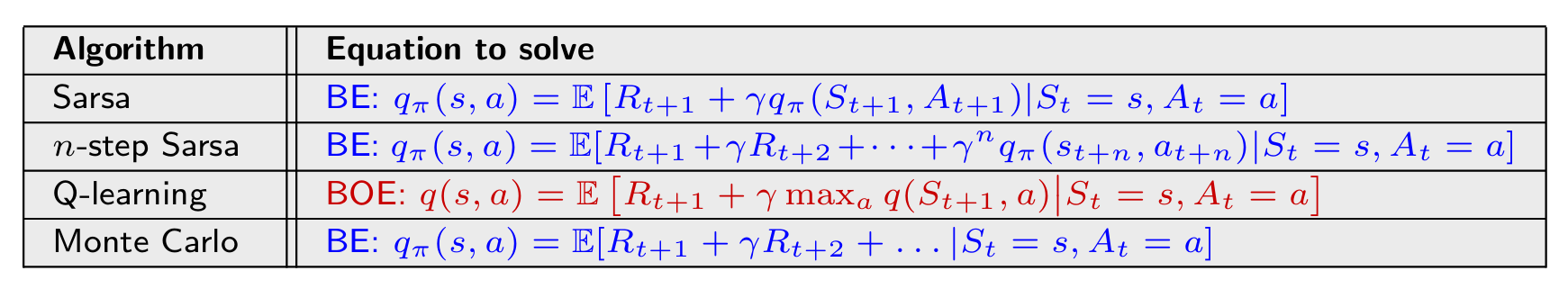
2. Sarsa

TD Learning of Action Values，功能为 Policy Evaluation

• 可以估计 Action Value

• 可以搜索 Optimal Policy

  因为它终于开始涉及 Action 了，能评估不同 Action 的效果（求 Action Value），就能设法用 $\epsilon$-Greedy 的方式去选出合适的 Action 来更新 Policy

 

 

2.1 Problem Formulation

• Given

  1. Policy $\pi$

  2. Experience Samples generated by $\pi$ in the form

     State, Action, Reward, State, Action = SARSA

• Task

  Estimate Action Values $\{q_{\pi}(s, a)\}_{s\in\mathcal{S}, a\in\mathcal{A}}$ under $\pi$

 

 

2.2 Sarsa

相当于 Action Value 版本的 TD(0)

• Mathematical Objective

  a stochastic approximation algorithm solving

  这是一种 BEE 用 Action Value 表达的写法

• Algorithm

  每次 Update Action Value 需要的 Experience 为一组 $\{ s_t, a_t, r_{t+1}, s_{t+1}, a_{t+1}\}$

  where

  • $s_t\longrightarrow$ The visited State at Time Step $t$
  • $a_t \longrightarrow$ The selected Action at Time Step $t$
  • $q_t(s_t, a_t) \longrightarrow$ Estimation of Action Value $q_{\pi}(s_t, a_t)$, or "Q-Table"
  • $\alpha_t(s_t)\longrightarrow$ Learning Rate depending on $s_t, a_t$ at Time Step $t$ (a small positive number)

• Pseudo-Code

  In general, we maintain a Q-Table $q(s,a)$ outside the episodes

  $\epsilon$-Greedy Update 方式此处不细讲了，在某 State $s_n$ 选择 Action 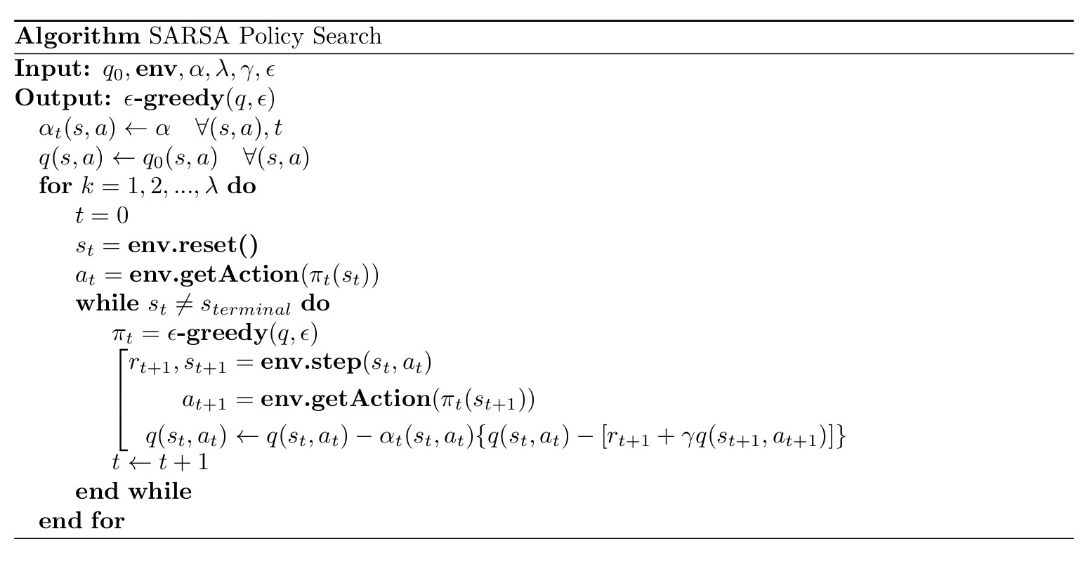$a$ 的条件是 $a = \arg\max_a q(s_n, a)$

  

 

 

2.3 Expected Sarsa

与一般版本的 Sarsa 的区别在于 TD Target 稍微变了一下

这样能将每组 Experience 涉及的 Random Variable 减少

• Matwhematical Objective

  a stochastic approximation algorithm solving

  这是也一种 BEE 用 Action Value 表达的写法

• Algorithm

  每次 Update Action Value 需要的 Experience 为一组 $\{ s_t, a_t, r_{t+1}, s_{t+1}\}$

• Notes

  1. Needs more computation
  2. 由于减少了涉及的 Random Variable，所以能 reduce estimation variances

 

 

2.4 n-Step Sarsa

这是个介于 2.2 的一般 Sarsa 和 Monte-Carlo 之间的算法，关键在 Action Value 的公式上

• Intuition

  Discounted Return $G_t$ can be written in different form as

  [ WARNING ]

  请千万记住，以上只是 written in different forms！

  所有的 superscript 都只是用于表示 $G_t$ 的分解程度

• Mathematical Objective

  • Sarsa

    It aims to solve

  • Monte-Carlo

    It aims to solve

  • n-Step Sarsa

    It aims to solve

    • n-Step Sarsa = Sarsa, when $n = 1$
    • n-Step Sarsa = Monte-Carlo, when $n = \infin$

• Algorithm

  每次 Update Action Value 需要的 Experience 为一组 $\{ s_t, a_t, r_{t+1}, s_{t+1}, a_{t+1}, \cdots, r_{t+n}, s_{t+n}, a_{t+n}\}$

  We need to wait until Time Step $n+1$ to update Action Value of $(s_t, a_t)$

• Notes

  Performance is a blend of Sarsa and Monte-Carlo

  • if n is large, then it has a large variance but a small bias
  • if n is small, then it has a large bias but a small variance

 

 

 

3. Q-Learning

TD Learning of Optimal Action Values

和 Sarsa 很像，但 TD Target 以及做 Policy Improvement 时所用方法的区别非常大

 

 

3.1 Algorithm

• Mathematical Objective

  It aims to solve

  This is a BOE instead of BEE expressed in terms of Action Values!

  所以 Q-Learning 能直接 estimate (optimal policy 对应的) optimal action value

• Algorithm

  每次 Update Action Value 需要的 Experience 为一组 $\{ s_t, a_t, r_{t+1}, s_{t+1}\}$

  不需要 $a_{t+1}$ 的原因是，它应该是通过 $\max_{a\in\mathcal{A}}$ 得到的

• Notes

  Q-Learning 有 (类) On-Policy 和 Off-Policy 两种版本

 

 

3.2 On-Policy Ver. Pseudo-Code

$\epsilon$-Greedy Update 方式此处不细讲了，在某 State $s_n$ 选择 Action $a$ 的条件是 $a = \arg\max_a q(s_n, a)$

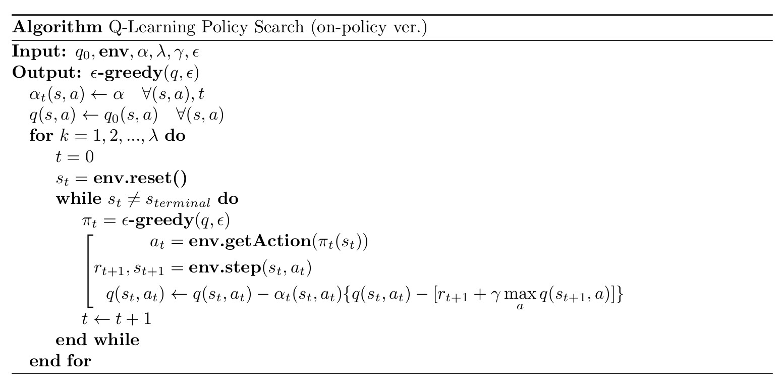
请注意它本质上是类似 on-policy

 

 

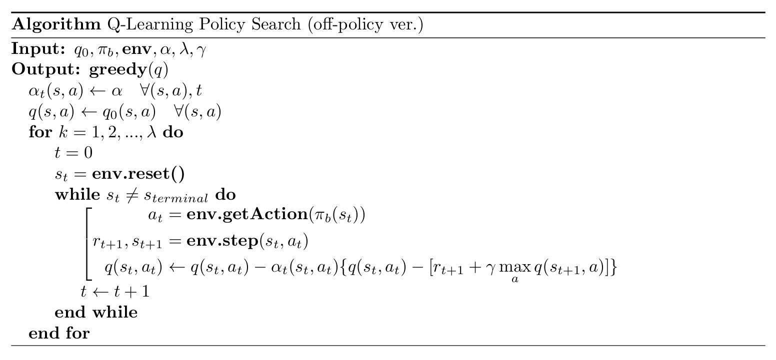
3.3 Off-Policy Ver. Pseudo-Code

请注意，Off-Policy Learning 的算法在 Update Policy 时不需要考虑 Target Policy $\pi_T$ 的探索性（探索交给 Behavior Policy $\pi_b$）

所以在 Update Target Policy 的时候，可以舍弃 $\epsilon$-Greedy 而直接用 Greedy 的方式更新

对于某个 State $s_n$，Greedy Update 的方式为 $\pi_{T}(a|s_n) = [a = \arg\max_a q(s_n, a)]$ ? 1 : 0

以下为 Pseudo Code

 

 

 

[ Notes ] Universal Expression

• Algorithm

  

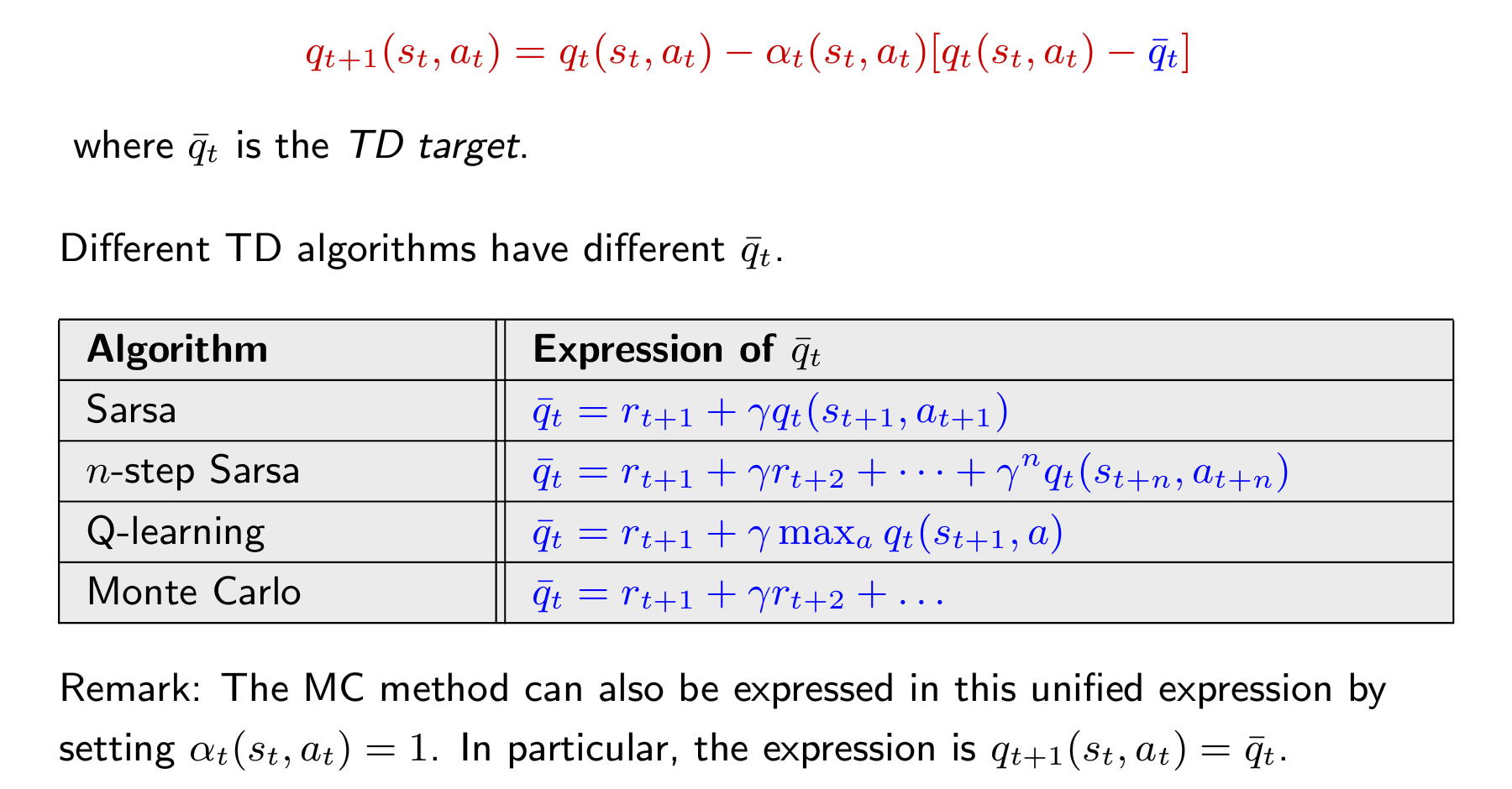
• Mathematical Objective

  

 

 

 

[ Notes ] On/Off-Policy Learning

Temporal-Difference Learning 的算法涉及 Generate Experience 和 Optimize Policy 两件事

• Behavior Policy is used to Generate Experience Samples
• Target Policy is constantly updated towards Optimal Policy

所谓 On-Policy 与 Off-Policy 的区别便在于这两种 Policy 是否一致

• On-Policy Learning $\longrightarrow$ Behavior Policy $=$ Target Policy

  Policy 先被用来 Generate Experience，然后 Optimize，这两个步骤不断循环

• Off-Policy Learning $\longrightarrow$ Behavior Policy $\not=$ Target Policy

  Policy A 专门用来 Generate Experience，用来 Optimize Policy B

比如 Sarsa 和 Monte-Carlo 都是 On-Policy，Q-Learning 一般是 Off-Policy 的，但也可以被 implement 成类似 On-Policy 的形式

 

 

 

Special Topics - Robbins-Monro

这个 RM Algorithm 是 Temporal Difference Method 的基础

 

1. Algorithm

一种用于 Stochastic Approximation 的算法

• Problem Formulation

  很多问题都能写成这种形式：find the Root $w$ of equation $g$ that satisfies

  解的时候有两种情况：

  1. Model-Based

     即已知 $g$ 是什么，那么就会有各种 Numerical Method 任君挑选

  2. Model-Free

     即未知 $g$ 是什么，那么就用 Robbins-Monro (RM) Algorithm 来解

• Algorithm

  where

  • $w_k \longrightarrow k^{th}$ estimation of root
  • $\times a_k\longrightarrow$ 某 Positive Coefficient
  • $\eta_k\longrightarrow$ 观测时的 Noise，不理解可见 3.1 的例子
  • $\tilde{g}(w_k,\eta_k) = g(w_k) + \eta_k \longrightarrow$ Noisy Observation

  还是那句话：没 Model 就得有 Data，没 Data 就得有 Model

• Example

  Assume parameters

  • $w_1 = 3$
  • $a_k = 1/k$
  • $\eta_k = 0 \longrightarrow$ 即假设没有 Noise，$\tilde{g}(w_k,\eta_k)=g(w_k)$

  则 RM Algorithm 为

  迭代效果如下图

  

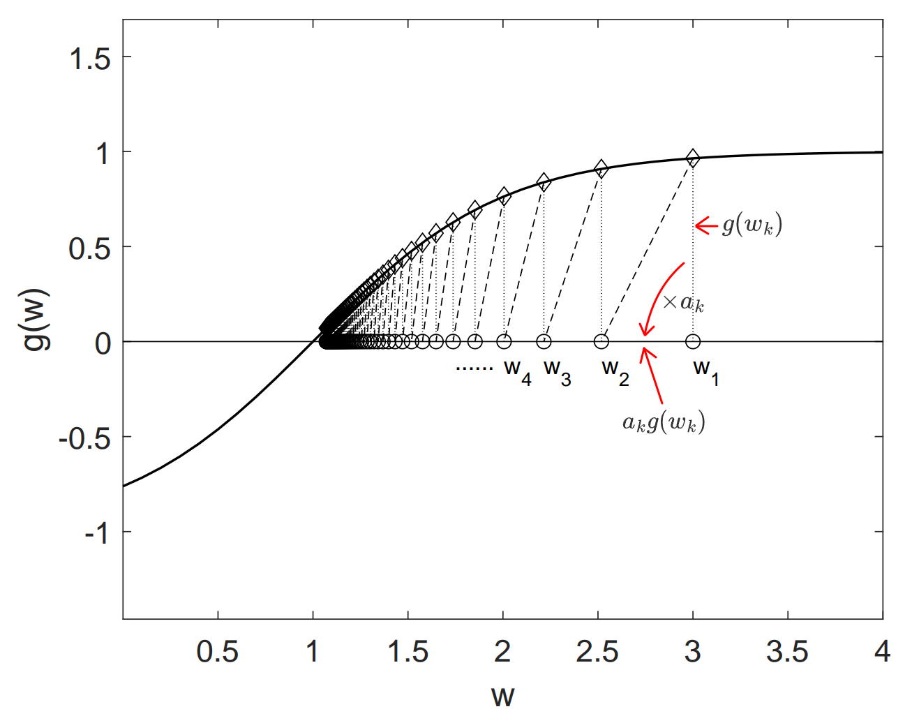
  实际上无论初始值的正负如何，最后总是能迭代收敛到 True Root $w^* = 1$

 

 

 

2. Convergence Theorem

In RM Algorithm, if

• $0 < c_1 \leq \grad_wg(w) \leq c_2$

  即 $g$ 的图像始终递增且梯度有界，这样能确保一定有 $g(w^*)=0$

• $\sum_{k=1}^{\infin}a_k = \infin$ and $\sum_{k=1}^{\infin}a_k^2 < \infin$

  后者确保 "$a_k\to 0$ as $k\to \infin$"，前者确保 "$a_k$ 不会收敛得太快"

• $\mathbb{E}[\eta_k|\mathcal{H}_k]=0$ and $\mathbb{E}[\eta_k^2|\mathcal{H}_k]<\infin$ where $\mathcal{H}_k = \{w_k,w_{k-1},...\}$

  前者表示 "$\eta_k$ 的 mean 为 0"，后者表示 "$\eta_k$ 有界"，noise 不一定非要是 Gaussian

then $w_k$ converges with probability 1 (w.p.1) to the root $w^*$ satisfying $g(w^*)=0$

“with probability 1” 表示的是概率意义上的收敛，因为涉及随机变量采样

 

 

 

3. More Examples

走过路过，不要错过！Mean Estimation！

 

 

3.1 嗯...

Solve for $w$ with Independent & Identically Distributed Samples $\{x\}$ of $X$

Reformulate the problem to

得到的 Samples $\{x\}$ of $X$ 相当于是 Noisy Observation

where the Noise is

那么 RM Algorithm Formulation 为

 

3.2 哦吼吼～

增加点难度～

Solve for $w$ with Independent & Identically Distributed Samples $\{x\}$ of $X$

Reformulate the problem to

得到的 Samples $\{x\}$ of $X$ 相当于是 Noisy Observation

where the Noise is

那么 RM Algorithm Formulation 为

 

3.3 《 你 好 》

再加点佐料～

Solve for $w$ with Independent & Identically Distributed Samples $\{x\}$ of $X$ and Samples $\{r\}$ of $R$

Reformulate the problem to

得到的 Samples $\{x\}$ of $X$ 相当于是 Noisy Observation

where the Noise is

那么 RM Algorithm Formulation 为