Sequential Quadratic Programming

SQP = Sequential Quadratic Programming

这是一种处理 constrained nonlinear optimization 的算法，原理是直接对 KKT Conditions 使用 Newton’s Method

 

 

 

1. KKT Newton Step

以下是基本信息

• Lagrangian

• KKT Conditions

  展开后得到

 

 

1.1 Derivation

因为目的是用 Newtonian 去解能使 $\grad L(x, \lambda) = 0$ 的 $(x^*, \lambda^*)$，所以与 Optimal Control Basics 4.1.2 一样执行相同的步骤

对 KKT Condition 进行 1st-Order Taylor Expansion

since $\frac{\partial^2 L}{\partial x \partial \lambda} = \frac{\partial g}{\partial x}$ and $\frac{\partial g}{\partial \lambda} = 0$, then

重新组织一下，统一一下表述方式

变成 Discrete-Time Notation

变成 KKT System 矩阵

 

 

1.2 Summary

With

Solve for Step Direction $(\Delta x_k, \Delta \lambda_k)$, then the Newton Step is

好吧，update $x_{k+1}$ 的时候你是得考虑下 Step Length 的，不能真就这么相加了...

 

 

 

2. Step Direction

一般不会直接解 1.2 中的 KKT System 来得到 Step Direction，而是会进行一定程度的转化

 

 

2.1 Equivalent Matrix

重新整理第一行对应的公式

原先的 KKT System 就等同于

 

 

2.2 Equivalent QP

Consider a QP formulation of the following

• Lagrangian

• KKT Condition

• KKT System

好，现在和 2.1 中得到的 Equivalent Matrix 对比一下...

变量是可以对得上的

代入回 QP 中得到

Solve for $(p, \lambda)$ as the Step Direction

此时你甚至不需要再去考虑 $\lambda$ 要如何 update 了，因为 QP 解完就能直接得到下一个 Time Step 的 $\lambda_{k+1}$！

 

 

2.3 Summary

Solving the following KKT System

is equivalent to solving the following QP for $(p, \lambda)$

Inequality Constraints

很简单，只需要在 "subject to" 里面加一行，格式和 Equality Constraints 一样

where

• $\Delta x_k \longrightarrow$ Step Direction for $x_k$
• $\lambda_{k+1}\longrightarrow$ Lagrangian Multiplier at the next Time Step

 

 

 

3. Step Length

使用 Optimal Control Basics 2.2 中提到的 Backtracking Line Search，具体来说要用的是 Optimal Control Basics 2.2.1 的 Armijo / Sufficient Decrease Condition

• Regular Armijo

• Merit Function

  我们希望 Step Length 能 balance cost reduction & constraint satisfaction

  所以在 Sufficient Decrease Condition 中用 Merit Function $\phi(x)$ 代替 Optimization Objective $f(x)$

  Inequality Constraints

  增加一项即可

  关于 $\mu\norm{g(x)}_1$ 这一项

  • $\mu\longrightarrow$ Equality Constraint Violation Penalty
  • $\norm{g(x)}_1 \longrightarrow$ L1 Norm of $g(x)$
  • 目的是惩罚违反 Equality Constraint 的情况，即只要任何一个 $g_i(x) \not= 0$，其数值都会经由 $\mu$ 加入 Merit Function
  • 由于性质是 Penalty，所以等于是默许在早期的 Iteration 中可以轻微出现 Constraint Violation

• Merit-Based Armijo

  也顺带改成 Discrete-Time Notation，此处 Step Direction $p_k = \Delta x_k$

  • 由于 $\mu\norm{g(x)}_1$ 是纯粹的 Penalty，也没有也没法算标准的 gradient，所以就纯手动减了

  • Inequality Constraint

    同样的原理

 

 

 

4. Summary

• Step Direction

  Solve the following with any QP solver

  for $(p, \lambda)$, where Step Direction $\Delta x_k$ and Lagrangian Multiplier at the next Time Step $\lambda_{k+1}$ are

• Step Length

  Find Step Length $\alpha_k$ with Merit-Based Backtracking Line Search

  Define Merit Function

  Find a Step Length $\alpha_k$ that satisfies the Merit-Based Armijo Condition

  then update

 

 

 

 

 

Example

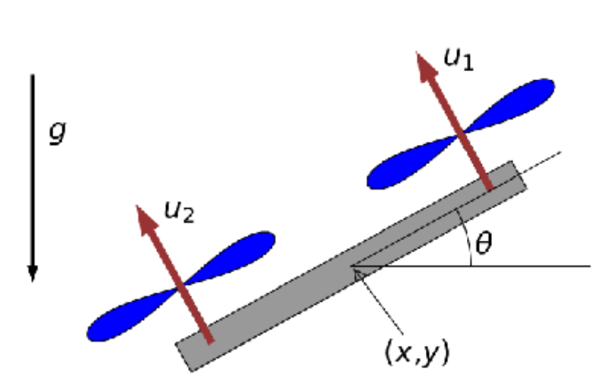
Formulation of a Sequential Quadratic Programming (SQP) problem to achieve flipping maneuvers for the following planar quadrotor

It is also desired to limit quadrotor thrust and quadrotor altitude

 

 

 

1. Quadrotor System Dynamics

 

 

 

2. Formulation of QP Subproblem

System Dynamics is first linearized using 1st-Order Taylor Expansion at $(x, u) = (\bar{x}, \bar{u}) + (\Delta x, \Delta u)$, and discretized at $(\Delta x, \Delta u)$ to form the QP Subproblem of SQP solver.

Equality Constraints is composed of system dynamics and initial conditions.

Inequality Constraints is composed of limitations on quadrotor thrust and limitations on quadrotor altitude.

 

 

2.1 Equality Constraints

 

2.1.1 Linearize the System

Rearrange the system dynamics

With guess trajectory $\bar{x}$, guess control $\bar{u}$, linearize the system using 1st-Order Taylor Expansion at $(\bar{x}, \bar{u})$

By assigning the following

we obtain a linear system in the form

Apply the above paradigm to the given nonlinear system, we have

 

2.1.2 Discretize the System

Given system dynamics $\dot{x} = f(x, u)$, we can discretize it using Euler's Method

Hence, for the linearized system in the previous section, we have

and in matrix form

Or simply in the form of the following equation

 

2.1.3 Constraint Formulation

The equality constraints are the initial conditions and the linearized system dynamics

and could be rewritten to the form

where $I\in \mathbb{R}^{6\times 6}$ and

 

 

2.2 Inequality Constraints

We need to

1. maintain the thrust of each rotor between 0 and 10
2. maintain the quadrotor at positive altitude

Therefore,

By assigning the following

The constraint could be linearized to

rearrange the terms to the form

The full matrix of inequality constraints are

 

 

 

3. SQP Cost Function

Cost function is formulated as the following with $Q$ as the state weight matrix and $R$ as the control weight

where the desired terminal trajectory $s_{des} = (x_{des}, u_{des})^T$ is

and we assign